Hey Everyone!

Today we'll be talking about

• How Benchling Quickly Compares DNA Strands with Millions of Base Pairs

  • Benchling is a biotech company that builds a platform for scientists to store, analyze and track research data

  • Their platform needs to be able to quickly compare DNA strands with millions of base pairs

  • They do this with Suffix trees, a data structure that is very commonly used for comparing strings

  • We’ll delve into the problem Benchling is solving, potential solutions, what a Suffix tree is and how you can use it

• Introduction to Storage Systems in Big Data Architectures

  • OLTP Databases and their key properties

  • Data Warehouses, Cloud Data Warehouses and ETL

  • Data Lakes and Data Swamps

  • The Data Lakehouse Pattern

• Tech Snippets

  • How to Burn out as a Software Engineer in 3 Easy Steps!

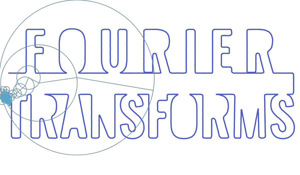
  • An Interactive Introduction to Fourier Transforms

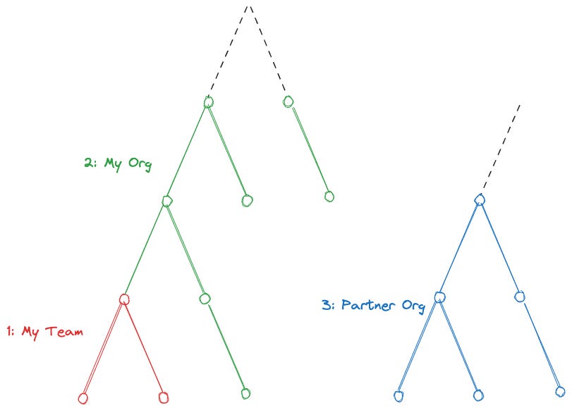
  • Tips from a Staff Engineer on Setting Cross-Team Workstreams

  • Paul Graham’s Latest Essay on Achieving Superlinear Returns

  • Imaginary Problems Are the Root of Bad Software

How Large Language Models Work

If you’re curious about how LLMs like GPT-4, LLaMA and Claude work then you should check out this fantastic course by Brilliant.

It’s fully interactive with animations, hands-on graphics and detailed explanations on things like

• N-Gram Models

• Transformers

• Fine Tuning LLMs

And more.

Brilliant is an education platform that has a huge amount of math, data sciennce, computer science and ML content. Their content is structured as bite-sized lessons with tons of interactive animations, graphics and more.

This makes it really easy to build a daily learning habit with the Brilliant app, instead of wasting time on Instagram or Twitter.

With the link below, you can get a 30-day free trial to check it out. You’ll also get a 20% discount when you subscribe.

sponsored

How Benchling Quickly Compares DNA Strands with Millions of Base Pairs

Benchling is a biotech startup that is building a cloud platform for researchers in the biology & life sciences field. Scientists at universities/pharmaceutical companies can use the platform to store/track experiment data, analyzing DNA sequences, collaboration and much more.

You can almost think of Benchling as a Google Workspace for Biotech research. The company was started in 2012 and is now worth over $6 billion dollars with all of the major pharmaceutical companies as customers.

A common workflow in biotech is molecular cloning, where you

1. Take a specific segment of DNA you’re interested in

2. Insert this DNA fragment into a plasmid (a circular piece of DNA)

3. Put this into a tiny organism (like a bacteria)

4. Have the bacteria make many copies of the inserted DNA as they grow and multiply

To learn more about DNA cloning, check out this great article by Khan Academy.

With molecular cloning, one important tool is homology-based cloning where a scientist will take DNA fragments with matching ends and join them together.

As a quick refresher, DNA is composed of four bases: adenine (A), thymine (T), guanine (G) and cytosine (C). These bases are paired together with adenine bonding with thymine and guanine bonding with cytosine.

You might have two DNA sequences. Here are the two strands (a strand is just one side of the DNA sequence):

1. 5'-ATGCAG-3'

2. 5'-TACGATGCACTA-3'

With homology-based cloning, the homologous region between these two strings is ATGCA. This region is present in both DNA sequences.

Finding the longest shared region between two fragments of DNA is a crucial feature for homology-based cloning that Benchling provides.

Karen Gu is a software engineer at Benchling and she wrote a fantastic blog post delving into molecular cloning, homology-based cloning methods and how Benchling is able to solve this problem at scale.

In this summary, we’ll focus on the computer science parts of the article because

1. This is a software engineering newsletter

2. I spent some time researching molecular cloning and 99.999% of it went completely over my head

Finding Common DNA Fragments

To reiterate, the problem is that we have DNA strands and we want to identify fragments in those strands that are the same.

With our old example, it is ATGCA

3. 5'-ATGCAG-3'

4. 5'-TACGATGCACTA-3'

Many of the algorithmic challenges you’ll have to tackle can often be simplified into a commonly-known, well-researched problem.

This task is no different, as it can be reduced to finding the longest common substring.

The longest common substring problem is where you have two (or more) substrings, and you want to find the longest substring that is common to all the input strings.

So, “ABABC” and “BABCA” have the longest common substring of “ABC“.

There’s many ways to tackle this problem, but three commonly discussed methods are

• Brute Force - Generate all substrings of the first string. For each possible substring, check if it’s a substring of the second string.
  If it is a substring, then check if it’s the longest match so far.
  
  This approach has a time complexity of O(n^3), so the time taken for processing scales cubically with the size of the input. In other words, this is not a good idea if you need to run it on long input strings.
  

• Dynamic Programming - The core idea behind Dynamic Programming is to take a problem and run divide & conquer on it. Break it down into smaller subproblems, solve those subproblems and then combine the results.
  
  Dynamic Programming shines when the subproblems are repeated (you have the same few subproblems appearing again and again). With DP, you cache the results of all your subproblems so that repeated subproblems can be solved very quickly (in O(1)/constant time).
  
  Here’s a fantastic video that delves into the DP solution to Longest Common Substring. The time complexity of this approach is O(n^2), so the processing scales quadratically with the size of the input. Still not optimal.
  

• Suffix Tree - Prefix and Suffix trees are common data structures that are incredibly useful for processing strings.
  
  A prefix tree (also known as a trie) is where each path from the root node to the leaf node represents a specific string in your dataset. Prefix trees are extremely useful for autocomplete systems.
  

  

  
  
  A suffix tree is where you take all the suffixes of a string (a suffix is a substring that starts at any position in the string and goes all the way to the end) and then use all of them to build a prefix tree.

  
  For the word BANANA, the suffixes are

  • BANANA

  • ANANA

  • NANA

  • ANA

  • NA

  • A

  
  Here’s the suffix tree for BANANA where $ signifies the end of the string.
  

  

Solving the Longest Common Substring Problem with a Suffix Tree

In order to solve the longest common substring problem, we’ll need a generalized suffix tree.

This is where you combine all the strings that you want to find the longest common substring of into one big string.

If we want to find the longest common substring of GATTACA, ATCG and ATTAC, then we’ll combine them into a single string - GATTACA$ATCG#ATTAC@ where $, # and @ are end-of-string markers.

Then, we’ll build a suffix tree using this combined string (this is the generalized suffix tree as it contains all the strings).

As you’re building the suffix tree, mark each node with which input string the leaf node corresponds to. This way, you know which nodes contain all the input strings, a few of the input strings, or only one input string.

Once you build the generalized suffix tree, you need to perform a depth-first search on this tree, where you’re looking for the deepest node that contains all the input strings.

The path to this deepest node (the sequence of nodes from the root to this deepest node) is your longest common subsequence.

Building the generalized suffix tree can be done with Ukkonen’s algorithm, which runs in linear time (O(n) where n is the length of the combined string). Doing the depth-first search also takes linear time.

This method performs significantly better but Benchling still runs into limits when the length of the DNA strands contain millions of bases.

They plan on optimizing further by implementing the algorithm in C (they’re currently using Python) and also by delving into faster techniques for finding the Longest Common Substring.

For more details, please read the full article here.

How Large Language Models Work

If you’re curious about how LLMs like GPT-4, LLaMA and Claude work then you should check out this fantastic course by Brilliant.

It’s fully interactive with animations, hands-on graphics and detailed explanations on things like

• N-Gram Models

• Transformers

• Fine Tuning LLMs

And more.

Brilliant is an education platform that has a huge amount of math, data sciennce, computer science and ML content. Their content is structured as bite-sized lessons with tons of interactive animations, graphics and more.

This makes it really easy to build a daily learning habit with the Brilliant app, instead of wasting time on Instagram or Twitter.

With the link below, you can get a 30-day free trial to check it out. You’ll also get a 20% discount when you subscribe.

sponsored

Tech Snippets

An Introduction to Storage Systems in Big Data Architectures

This is an excerpt from our last Quastor Pro article on Big Data Architectures.

With Quastor Pro, you also get weekly deep dives on topics in building large scale systems (in addition to the blog summaries).

If you’re interested in mid/senior-level roles at Big Tech companies, then Quastor Pro is super helpful for system design interviews.

You should be able to expense Quastor Pro with your job’s learning & development budget. Here’s an email you can send to your manager.

In past Quastor articles, we’ve delved into big data architectures and how you can build a system that processes petabytes of data.

We’ve discussed how

• Shopify ingests transaction data from millions of merchants for their Black Friday dashboard

• Pinterest processes and stores logs from hundreds of millions of users to improve app performance

• Facebook analyzes and stores billions of conversations from user device microphones to generate advertising recommendations (Just kidding. Hopefully they don’t do this)

In these systems, there are several key components:

• Sources - origins of data. This can be from a payment processor (Stripe), google analytics, a CRM (salesforce or hubspot), etc.

• Integration - transfers data between different components in the system and minimizes coupling between the different parts. Tools include Kafka, RabbitMQ, Kinesis, etc.

• Storage - store the data so it’s easy to access. There’s many different types of storage systems depending on your requirements

• Processing - run calculations on the data in an efficient way. The data is typically distributed across many nodes, so the processing framework needs to account for this. Apache Spark is the most popular tool used for this; we did a deep dive on Spark that you can read here.

• Consumption - the data (and insights generated from it) gets passed to tools like Tableau and Grafana so that end-users (business intelligence, data analysts, data scientists, etc.) can explore and understand what’s going on

In this Quastor Pro article, we’ll delve into storage.

We’ll be talking about

• OLTP databases

• Data Warehouses

• Data Lakes

• Data Lakehouses

We’ll have a ton of buzzwords in this article, so don’t forget to fill out your Buzzword Bingo scorecards as you read this article. First person to reply with BINGO gets a prize 😉.

OLTP Databases

OLTP stands for Online Transaction Processing. This is your relational/no-sql database that you’re using to store data like customer info, recent transactions, login credentials, etc.

Popular databases in this category include Postgres, MySQL, MongoDB, DynamoDB, etc.

The typical access pattern is that you’ll have some kind of key (user ID, transaction number, etc.) and you want to immediately get/modify data for that specific key. You might need to decrement the cash balance of a customer for a banking app, get a person’s name, address and phone number for a CRM app, etc.

Based on this access pattern, some key properties of OLTP databases are

• Real Time - As indicated by the “Online” in OLTP, these databases needs to respond to queries within a couple hundred milliseconds.

• Concurrency - You might have hundreds or even thousands of requests being sent every minute. The database should be able to handle these requests concurrently and process them in the right order.

• Transactions - You should be able to do multiple database reads/writes in a single operation. Relational databases often provide ACID guarantees around transactions.

• Row Oriented - We have a detailed article delving into row vs. column oriented databases here but this just refers to how data is written to disk. Not all OLTP databases are row oriented but examples of row-oriented databases include Postgres, MySQL, Microsoft SQL server and more.

OLTP databases are great for handling day-to-day operations, but what if you don’t have to change the data? What if you have a huge amount of historical read-only data that you need for generating reports, running ML algorithms, archives, etc.

This is where data warehouses and data lakes come into play.

Data Warehouse

Instead of OLTP, data warehouses are OLAP - Online Analytical Processing. They’re used for analytics workloads on large amounts of data.

Data warehouses hold structured data, so the values are stored in rows and columns. Data analysts/scientists can use the warehouse for tasks like analyzing trends, monitoring inventory levels, generating reports, and more.

Using the production database (OLTP database) to run these analytical tasks/generate reports is generally not a good idea.

You need your production database to serve customer requests as quickly as possible.

Analytical queries (like going through every single customer transaction and aggregating the data to calculate daily profit/loss) can be extremely compute-intensive and the OLTP databases aren’t designed for these kinds of workloads.

Having data analysts run compute-intensive queries on the production database would end up degrading the user experience for all your customers.

OLAP databases are specifically designed to handle these tasks.

Therefore, you need a process called ETL (Extract, Transform, Load) to

1. Extract the exact data you need from the OLTP database and any other sources like CRM, payment processor (stripe), etc.

2. Transform it into the form you need (restructuring it, removing duplicates, handling missing values, etc.). This is done in your data pipelines or with a tool like Apache Airflow.

3. Load it into the data warehouse (where the data warehouse is optimized for complex analytical queries)

The key properties of data warehouses are

• Column Oriented - We mentioned that OLTP databases are row-oriented. This means that all the data from the same row is stored together on disk.
  
  Data warehouses (and other OLAP systems) are generally column-oriented, where all the data from the same column is stored together on disk. This minimizes the number of disk reads when you want to run computations on all the values in a certain column.
  
  We did a deep dive on Row vs. Column oriented databases that you can check out here.

• Highly Scalable - Data warehouses are designed to be distributed so they can scale to store terabytes/petabytes of data

Cloud Data Warehouses

Prior to 2010, only large, sophisticated companies had data warehouses. These systems were all on-premises and they cost millions of dollars to install and maintain (i.e. this is why Larry Ellison is worth $160 billion dollars).

This changed in 2012 with AWS Redshift and Google BigQuery. Snowflake came along in 2014.

Now, you could spin up a data warehouse in the cloud and increase/decrease capacity on-demand. Many more companies have been able to take advantage of data warehouses by using cloud services.

With the rise of Cloud Data warehouses, an alternative to ETL has become popular - ELT (Extract, Load, Transform)

1. Extract the data you need from all your sources (this is the same as ETL)

2. Load the raw data into a staging area in your data warehouse (Redshift calls this a staging table)

3. Transform the data from the staging area into all the different views/tables that you need.

This is the first part of the Quastor Pro article on storage systems. In the next part, we’ll talk about Pros/Cons of ELT vs. ELT, Data Lakes, Data Swamps, the Data Lakehouse pattern and more.

You should be able to expense Quastor Pro with your job’s learning & development budget. Here’s an email you can send to your manager.

Past Quastor Pro Content

System Design Topics

• Measuring Availability

• API Gateways

• Database Replication and Sharding

• Load Balancing Strategies

• API Paradigms

• Backend Caching Strategies

• Event Driven Architectures

• Consistency Models

• DNS Explained

Tech Dives

• Apache Kafka

• DynamoDB

• HTTP

• gRPC

• Apache Spark

• Google File System

• Map Reduce

• Chaos Engineering

Databases

• A Dive Into the CAP Theorem

• B Trees vs. LSM Trees

• Page Oriented Storage Engines and B Trees

• Log Structured Storage Engines

• Database Storage Engines

• Row vs. Column Oriented Databases